Defining lattice models
This section explains how to define lattice models through python calls.
A simple example
The following simple example illustrates how to define a Hubbard model on the square lattice in two dimensions:
import pyqcm

CM = pyqcm.cluster_model(4, 0, 'clus', ((4, 3, 2, 1),))
clus = pyqcm.cluster(CM, ((0, 0, 0), (1, 0, 0), (0, 1, 0), (1, 1, 0)))
model = pyqcm.lattice_model('2x2_C2', clus, ((2, 0, 0), (0, 2, 0)))
model.interaction_operator('U')
model.hopping_operator('t', (1, 0, 0), -1)
model.hopping_operator('t', (0, 1, 0), -1)
model.hopping_operator('t2', (1, 1, 0), -1)
model.hopping_operator('t2', (-1, 1, 0), -1)
model.hopping_operator('t3', (2, 0, 0), -1)
model.hopping_operator('t3', (0, 2, 0), -1)
model.anomalous_operator('D', (1, 0, 0), 1)
model.anomalous_operator('D', (0, 1, 0), -1)
model.density_wave('M', 'Z', (1, 1, 0))
There is a call to cluster_model() to define a \(2\times2\) plaquette with a \(C_2\) symmetry (rotation by 180 degrees). Then another object, of type cluster, is defined based on this model. This object has geometrical meaning, whereas the cluster_model does not. The cluster constructor takes the following arguments:
The
cluster_modelobject it is based on. It is possible to associate more than one cluster model to a cluster, if one wants to use the subbath concept is dynamical mean field theory.An array of integer positions of the different cluster sites. This is where the geometry of the cluster appears.
The base position of the cluster within the super unit cell (
[0,0,0]by default). This is just added for convenience when complex super unit cells are built out of the same cluster, shifted in position.
Once the different clusters (or the single cluster) have been defined, one can construct an object of type lattice_model that contains the different clusters arranged in a super-lattice. The constructor takes the following arguments:
The name of the model, for reporting purposes
The cluster (or sequence of clusters) forming the repeated unit.
The \(d\) vectors defining the superlattice vectors. \(d\) is the dimension of the model.
The \(d\) vectors defining the lattice vectors of the model. In the above example this is omitted because the default value is used:
((1,0,0), (0,1,0)).
Note that all vectors used in these specifications have three components (even for lower dimensional models) and have integer components. They are in fact coefficients of basis vectors generating a working Bravais lattice and are therefore integers by definition (not all vectors of this working Bravais lattice need belong to the actual Bravais lattice of the model; the case of the graphene lattice is illustrated below). They can be tuples, lists or numpy arrays. We recommend using tuples for simplicity.
Once the geometry of the model is defined, operators can be added to the model via various functions. The Hubbard on-site interaction is added with a call to the lattice_model member function interaction_operator('U'), whose sole argument in this case is the name we choose for that operator (more arguments are needed for other types of interactions, multi-band models, etc; see the detailed documents in the reference section on functions).
Nearest-neighbor hopping is defined with a call to the member function hopping_operator(), which has three mandatory arguments:
The name of the operator
The link on which the operator is defined
The amplitude of the operator on that link.
Optional keyword arguments are needed for multi-band models, spin-flip operators, etc. In the above example this function is called twice with the same name but different links (along (1,0,0) and (0,1,0) respectively). The matrix elements generated by the two calls are simply added to the list associated with this operator. Similar calls are performed for the second-neighbor hopping t2 and the third-neighbor hopping t3.
A d-wave pairing operator is defined via a call to anomalous_operator() , which takes the same arguments as hopping_operator(), i.e., name, link and amplitude. Note that two calls are made with the same name D, one in the \(x\) direction, the other one in the \(y\) direction, with amplitudes 1 and -1, in accordance with the d-wave character of the operator.
Finally, a density wave corresponding to \((\pi,\pi)\) antiferromagnetism is added, with a call to density_wave(), which has 3 mandatory arguments:
The name of the operator (here ‘M’)
- The type of density-wave (here ‘Z’ for a spin density wave in the \(z\) component of the spin). Other possibilities are:
‘N’ : charge density wave
‘X’ : spin density wave in the \(x\) component of the spin
‘spin’ : same as Z
‘singlet’ : singlet pairing
‘dx’ : triplet pairing in the \(x\) direction using the \(\mathbf{d}\) vector formalism.
‘dy’ : same, in the \(y\) direction
‘dz’ : same, in the \(z\) direction (this one does not require Nambu doubling)
The wavevector \(\mathbf{Q}\) of the density wave. It has real components (in multiples of \(\pi\)) and it must be commensurate with the super unit cell within some small numerical tolerance.
Additional keyword arguments to density_wave() include the link on which the density wave is defined (for bond-density waves), lattice orbitals involved (for multi-band models), additional phases and amplitudes, etc. Again, see the reference section for details.
A more complex example
The following example defines a model on the graphene lattice using two clusters within the super unit cell and the graphene lattice, as illustrated below:
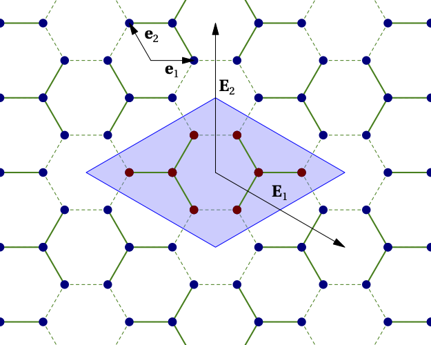
Figure 3
A possible set of function calls to define the Hubbard model on this system is:
from cluster_h4_6b_C3 import CM
import pyqcm

C1 = pyqcm.cluster(CM, [[0, 0, 0], [-1, 0, 0], [1, 1, 0], [0, -1, 0]], [-1, 0, 0])
C2 = pyqcm.cluster(CM, [[0, 0, 0], [1, 0, 0], [-1, -1, 0], [0, 1, 0]], [1, 0, 0])
model = pyqcm.lattice_model('h4_6b_C3', (C1, C2), [[2, -2, 0],[2, 4, 0]], [[1, -1, 0], [2, 1, 0]])
model.set_basis([[1, 0, 0], [-0.5, 0.866025403784438, 0], [0, 0, 1]])

model.interaction_operator('U')
model.hopping_operator('t', [1,0,0], -1, orbitals=(2,1))
model.hopping_operator('t', [0,1,0], -1, orbitals=(2,1))
model.hopping_operator('t', [-1,-1,0], -1, orbitals=(2,1))
The first statement, from cluster_h4_6b_C3 import CM, imports a cluster definition file, for instance the one associated with Fig. 2 above, in which the cluster_model object named CM was defined.
Two copies of the clusters are added to the super unit cell. The positions associated with the two copies are different, but the cluster model is the same, which means that only one copy of the Hilbert space operators and bases necessary for the exact diagonalization will be constructed. The origin has been placed exactly between the two clusters. The positions in each cluster are defined relative to the base position of each cluster.
The integer positions are defined in terms of the basis defined by the call to set_basis(). The argument of that function is a set of real-valued vectors defining the basis vectors of the working Bravais lattice.
On Fig. 3, the first two of these vectors are \(\mathbf{e}_1\) and \(\mathbf{e}_2\).
The call to lattice_model() defines both the superlattice vectors \(\mathbf{E}_1\) and \(\mathbf{E}_2\) (second argument) and the basis vectors of the model’s physical Bravais lattice (third argument).
The lattice basis vectors only serve to attribute orbital labels to the different sites. In qcm, each degree of freedom of a given spin (i.e. each orbital) must have its own site on the working Bravais lattice. The basis vectors of the physical Bravais lattice then define orbital labels (from 1 to \(N_\mathrm{band}\)) attributed to each site. The order in which orbitals are labelled depends on the order in which the sites appear. Given the above definitions and Fig. 3, the A sublattice of graphene corresponds to orbital 2 and the B sublattice to orbital 1.
Given that the model has two bands, the definition of the hopping operator t must contain orbital information: the keywords orbitals (a tuple) is used to specify the orbital numbers associated with the two sites separated by the bond vector (link) given in argument. Internally, a loop is done over all sites of the super unit cell; the bond vector is used to identify a second site; if that site exists and if the orbitals associated with the two sites agree with orbitals, then a matrix element is added to the operator. In the above example, three calls are needed because of the three directions (bonds).
The greatest risk in such calls is to mislabel the orbitals. In order to check that operators were defined properly, a
submodule called draw_operator is provided, that can draw on the screen a schematic view of each operator defined on the lattice or in a particular cluster model.
Other examples
The distribution contains a folder (notebooks) that contains many examples of models and codes. New users are encouraged to study a few of these models and to consult the reference section for more detailed information about model building.
Class lattice_model
- class lattice_model(name, clus, superlattice, lattice=None, hybrid_file='')
Class containing the unique model studied by this library
- Parameters:
name (str) – a name given to the model, for reference in the output data
clus ([cluster]) – a single object or a sequence of objects of the class cluster, forming the repeated unit
superlattice (list[list[int]]) – the integer-component vectors defining the superlattice. Their number is the spatial dimension of the model.
lattice (list[list[int]]) – the the integer-component vectors defining the lattice. Used to define bands.
- hopping_operator(name, link, amplitude, orbitals=None, **kwargs)
Defines a hopping term or, more generally, a one-body operator
- Parameters:
- Keyword Arguments:
- Returns:
None
- anomalous_operator(name, link, amplitude, orbitals=None, **kwargs)
Defines an anomalous operator
- Parameters:
- Keyword Arguments:
type (str) – one of ‘singlet’ (default), ‘dz’, ‘dy’, ‘dx’
- Returns:
None
- explicit_operator(name, elem, **kwargs)
Defines an explicit operator
- Parameters:
- Keyword Arguments:
- Returns:
None
- density_wave(name, t, Q, **kwargs)
Defines a density wave
- Parameters:
- Keyword Arguments:
- Returns:
None
- set_basis(B)
Define the working basis in terms of a physical basis, i.e., provides a transformation matrix between the two.
- Parameters:
B – the basis (a (D x 3) real matrix)
- Returns:
None
- interaction_operator(name, link=None, orbitals=None, **kwargs)
Defines an interaction operator of type Hubbard, Hund, Heisenberg or X, Y, Z
- Parameters:
- Keyword Arguments:
- Returns:
None
- set_target_sectors(sec)
Sets the Hilbert space sectors in which to look for the ground state. Each sector is specified by a string of the form ‘Rx:Ny:Sz’ where x is the irreducible representation label (starts at 0), y is the number of electrons and z is twice the total spin projection. For instance, ‘R0:N7:S1’ means 7 electrons and total spin projection 1/2, in the trivial representation. If more than one sector must be explored, their corresponding strings are separated by ‘/’, e.g. ‘R0:N7:S1/R0:N7:S-1’.
- Parameters:
sec ((str)) – the target sectors
- Returns:
None
- set_parameters(params)
Defines a new set of parameters, including dependencies
- Parameters:
params (tuple/str) – the values/dependence of the parameters (array of 2- or 3-tuples), or string containing syntax (preferred method). See section in the documentation or examples for more details.
- set_parameter(name, value, pr=False)
sets the value of one or more parameter within a parameter_set
- set_multiplier(name, value, pr=False)
sets the multiplier value of a dependent parameter within a parameter_set. Also applied to a list.
- parameter_string(sys=None, CR=False, constr=False)
Returns a string with the model parameters. Used for including in plots. :param int sys: system label to print the parameters of (starts at 1). If 0, prints lattice parameters only. If None, prints all parameters. :param bool CR: if True, puts each parameter on a line. :param bool constr: if True, also includes constrained parameters
- parameters(param=None)
returns the values of the parameters in the parameter set, in the form of a dict, if p is None. if p is a list of parameter names, then returns an array of values associated (in the same order) to this list.
- Parameters:
param ([str]) – a list of parameter names (optional)
- Returns:
a dict {string,float} OR a numpy array of values
- parameter_set(opt='all')
returns the content of the parameter set
- Parameters:
opt (str) – governs the action of the function
- Returns:
depends on opt
if opt = ‘all’, all parameters as a dictionary {str,(float, str, float)}. The three components are
the value of the parameter,
the name of its overlord (or None),
the multiplier by which its value is obtained from that of the overlord.
if opt = ‘independent’, returns only the independent parameters, as a dictionary {str,float} if opt = ‘report’, returns a string with parameter values and dependencies.
- print_model(filename)
Prints a description of the model into a file
- Parameters:
filename (str) – name of the file
- Returns:
None
- set_params_from_file(out_file, n=0, pr=False)
sets the parameters in the parameter_set object from a file
- fidelity(I1, I2, clus=0)
computes the fidelity between the two instances I1 and I2, i.e. the overlap squared of the ground states (or generalization thereof in case of a mixed state)
- Parameters:
I1 (model_instance) – first model instance
I2 (model_instance) – second model instance
clus (int) – cluster label
- finalize()
Sets some data for the model following the first instance declaration e.g. the mixing state of the system:
0 – normal. GF matrix is n x n, n being the number of sites
1 – anomalous. GF matrix is 2n x 2n
2 – spin-flip. GF matrix is 2n x 2n
3 – anomalous and spin-flip (full Nambu doubling). GF matrix is 4n x 4n
4 – up and down spins different. GF matrix is n x n, but computed twice, with spin_down = false and true
- compact_tiling(A, k)
Symmetrizes a
dim_GFmatrix with respect to cluster translations at wavevector k.For each element \(A[s(x), s(x')]\) with link \(\mathbf{d} = x' - x\), the result is:
\[A_{\rm ct}[s(x), s(x')] = \frac{1}{L_c} \sum_y A[s(y),\, s(f(y+d))]\, e^{i\mathbf{k}\cdot\boldsymbol{\delta}}\]where \(f(y+d)\) folds \(y+d\) back into the super unit cell and \(\boldsymbol{\delta}\) is the wrapping superlattice vector.
- Parameters:
A – input matrix (ndarray of shape
(d, d), complex,d=dim_GF)k – wavevector (ndarray(3)) in the same convention as
tk(): \(k_{\rm phys}\,a/(2\pi)\), where \(a\) is the primitive lattice constant. The inter-cluster Bloch phase for wrapping vector \(\mathbf{R}\) (in primitive lattice units) is \(e^{i\mathbf{k}\cdot\mathbf{R}\,2\pi}\).
- Returns:
symmetrized matrix (ndarray of shape
(d, d), complex)
- periodize_matrix(A, k)
Periodizes a
dim_GFmatrix (Green function, CPT Green function or self-energy) into the reduced band-space matrix of dimensiondimGF_red(= nband * n_mixed), at wavevector k.- Parameters:
A – input matrix (ndarray of shape
(d, d), complex,d=dim_GF)k – wavevector (ndarray(3)) in the superdual basis (same convention as
compact_tiling())
- Returns:
periodized matrix (ndarray of shape
(dimGF_red, dimGF_red), complex)
- periodize_vector(v, k)
Periodizes a
dim_GFvector into the reduced band-space vector of dimensiondimGF_red(= nband * n_mixed), at wavevector k.- Parameters:
v – input vector (ndarray of shape
(d,), complex,d=dim_GF)k – wavevector (ndarray(3)) in the superdual basis (same convention as
compact_tiling())
- Returns:
periodized vector (ndarray of shape
(dimGF_red,), complex)
- write_definition(filename=None, str=False)
Writes a Python file containing the code necessary to define this lattice_model.
The generated file contains calls to cluster_model, cluster and lattice_model constructors and their operator-adding methods, reproducing the full model definition.
- draw_cluster_operator(sys, op_name, show_labels=True, values=False, spin_offset=0.15, plt_ax=None)
Draws an operator defined on a cluster model to the screen (for debugging purposes)
- Parameters:
sys (int) – label of a system
op_name (str) – name of the operator
show_labels (bool) – if True, shows the labels of the cluster
values (bool) – if True, prints de values of the elements
spin_offset (float) – graphical offset between up and down spins
plt_ax (matplotlib.axes.Axes) – optional matplotlib axis set, to be passed when one wants to collect a subplot of a larger set
- draw_operator(op_name, show_labels=False, show_orb_labels=True, show_neighbors=False, values=False, offset=0.05, orb_offset=0.05, z_offset=0.0, alpha_inter=0.2, spin_scale=0.1, plt_ax=None)
Draws an operator defined on a lattice model to the screen (for debugging purposes)
- Parameters:
op_name (str) – name of the operator
show_labels (bool) – if True, shows the labels of the cluster
show_neighbors (bool) – if True, shows the neighbors of the central cluster
values (bool) – if True, prints de values of the elements
offset (float) – offset between sites and labels
orb_offset (float) – offset between sites and orbital labels
z_offset (float) – offset between sites and labels for sites along the z axis
alpha_inter (float) – alpha value of the inter-cluster links
show_orb_labels (bool) – if True, shows the orbital index labels next to each site
spin_scale (float) – scale factor for the arrows representing spin polarization
plt_ax (matplotlib.axes.Axes) – optional matplotlib axis set, to be passed when one wants to collect a subplot of a larger set
- Hartree_procedure(task, couplings, maxiter=32, iteration='fixed_point', eps_algo=0, file='hartree.tsv', SEF=False, pr=False, alpha=0.0)
Performs the Hartree approximation
- Parameters:
task – task to perform within the loop. Must return a model_instance
couplings (hartree) – sequence of couplings (or single coupling), of the Hartree class
maxiter (int) – maximum number of iterations
iteration (str) – method of iteration of parameters (‘fixed_point’ or ‘broyden’)
eps_algo (int) – number of elements in the epsilon algorithm convergence accelerator = 2*eps_algo + 1 (0 = no acceleration)
file (str) – name of the file to which the converged result is written via write_summary()
SEF (bool) – if True, computes the Potthoff functional at the end of the procedure
pr (bool) – if True, prints progress of each coupling update
alpha (float) – if iteration=’fixed_point’, damping parameter, otherwise trial inverse Jacobian (if a float, that is (1+alpha)*unit matrix)
- Returns:
model instance, converged inverse Jacobian
- controlled_fade(task, P, n, C, file='fade.tsv', tol=0.0001, method='Broyden', maxiter=32, alpha=0.0, eps_algo=0, bracket=None, delta=None, verb=False)
Fades the model between two sets of parameters, in n steps
- Parameters:
task – task to perform within the loop
P (dict) – dict of parameters with a tuple of values (start and finish) for each
n – number of steps
C (dict) – dict of adjustable parameters whose average (the value of C) should stay fixed during the fade
file (str) – file to which the converged results are written
tol (float) – precision on the averages
method (str) – method used for solving the nonlinear constraints
maxiter – maximum number of iterations for solving the constraints
alpha (float) – parameter used in some non linear solvers (broyden)
eps_algo (int) – convergence accelerator parameter in fixed_point
bracket ((float,float)) – bracket used in some nonlinear 1D solvers
delta (float) – interval used to update the bracket used in some nonlinear 1D solvers
verb (bool) – If True, writes progress reports
- controlled_loop(task, varia=None, loop_param=None, loop_range=None, control_func=None, retry=None, max_retry=4, predict=True)
Performs a controlled loop for VCA or CDMFT with a predictor. The definition of each model instance must be done and returned by ‘task’; it is not done by this looping function.
- Parameters:
task – a function called at each step of the loop. Must return a model_instance.
varia ([str]) – names of the variational parameters
loop_param (str) – name of the parameter looped over
loop_range ((float, float, float)) – range of the loop (start, end, step)
control_func – (optional) name of the function that controls the loop (returns bool). Takes a model instance as argument
retry (char) – If None, stops on failure. If ‘refine’, adjusts the step (divide by 2) and retry. If ‘skip’, skip to next value.
max_retry (int) – Maximum number of retries of either type
predict (bool) – if True, uses a linear or quadratic predictor
- fade(task, P, n)
Fades the model between two sets of parameters, in n steps
- Parameters:
task – task to perform within the loop
P (dict) – dict of parameters with a tuple of values (start and finish) for each
n – number of steps
- Returns:
None
- linear_loop(N, task, varia=None, params=None, predict=True)
Performs a loop with a predictor. The definition of each model instance must be done in ‘task’; it is not done by this looping function.
- Parameters:
- Returns:
None
- loop_from_file(task, file)
Performs a task ‘task’ over a set of model parameters defined in a file. The definition of each model instance must be done in the task ‘task’; it is not done by this looping function.
- Parameters:
task – function (task) to perform
file (str) – name of the data file specifying the solutions, in the same tab-separated format usually used to write solutions
- loop_from_table(task, data)
Performs a task ‘task’ over a set of model parameters defined in a table. The definition of each model instance must be done in the task ‘task’; it is not done by this looping function.
- Parameters:
task – function (task) to perform
data (ndarray) – table of parameters, with named columns, as read or filtered from numpy.genfromtxt()
- model_instance()
Initiates a new instance of the lattice model :returns: A model_instance object